10 Best Excel Tools for Accountants

Spreadsheets have been around us for quite some time and they have been developed in to a handy tool. Some of them are propriety like Microsoft office and some can be used under creative commons license like open office. When it comes to collaboration or sharing data, google sheets take the top position.

You are going to read about 10 features of spreadsheets or Top 10 essential Excel Skills for accountants. (Adapted from Excel Zoom)

Use of Keyboard Shortcuts:

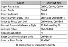You can also use built in short cut keys to perform certain action and if the option you are looking or is not available through shortcut keys! You can record also your own macros. Here are 10 shortcut keys that are most often used by excel user.

In recent version of MS Excel, you can invoke a hint to short cut keys but pressing Alt-Key from keyboard.

Presenting Data with Charts

It is always easy to understand data with Graphs.Here are some hints on using Excel Charts to make your reports interesting to read:

Use Bar and Line Charts – This is the best option if you want to plot time series data i.e. data over weeks, months and years. The bars clearly represent the plotted quantity and is really to read when it comes to comparison. (Shortcut keys: Bar Chart: Alt+N+C, Line Chart:Alt+N+L+N)

Use Pie Chart – when you want to show percentage of each component or breakup of something. You can use either absolute values or percentage. (Shortcut keys: Bar Chart: Alt+N+Q)

Scatter Plot – When you have data points and you want to explore the trend, just plot it using scatter plot. (Shortcut keys: Bar Chart: Alt+N+D)

Add a Trend line – Add a trend line to you Bar and Line Charts and your scatter plot, you can even get the expression and fit for the plotted data to understand the relationship.

Use Pivot Table to Summarize Data

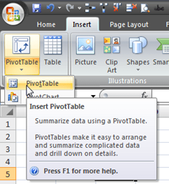When you have data in the form of list, the best option available to you to analyze it is a Pivot Table. With pivot table, you can manipulate data to great extend and you can be really quick in creating scenarios for your data.

You can insert a pivot table by using short cut key Alt+N+V. Add fields to Filter, Column, Rows and Values and select whether you want to sum, count or average the data. Besides built in functions, you can also create your own “Calculated Fields” and “Calculated Items” to shape your data.

Calculated Fields are Fields that are defined by formula – for example if commission on sales in 10%, you can create a new calculated field “Commission” by multiplying sales with 10% value. A calculated item is created by manipulating items in a given field.

Understand How Cell Referencing Works

There are four ways you can format your cell reference:

Keep row constant and column changeable –A$1, in this example, the $ before the row number (1 here) will keep it row one only. This is useful when you want drag formula downwards
Keep row moveable and column constant –$A1, in this example, the $ before the column number (A here) will keep it to one column only. This is useful when you want drag formula to right or left side.
Keep both row and column constant $A$1 – a dollar sign before both row and column means nothing can move.
Keep both row and column moveable – A1 this will make row and columns both moveable.

Understanding cell referencing style is important when you are using formulas across the worksheet and you want to refer to a cell a constant

Using Formula Auditing Toolbar:

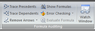Formulas are an essential part of spreadsheet. Large spreadsheet tend to contain error that can totally destroy the purpose of the sheet – some of the error are obvious and easily identify error and other are semantic error that tend to give you the result but an erroneous one. All of such formula activity can be checked for using the formula auditing tool bar.

The toolbar is present in Formula Tab. There is a whole bunch of options there to examine how formula is executed, to trace precedent and dependent cells and for tracing errors. Certainly this is one of the most useful features for accountants as they may want to create and then audit their own sheets.

Using Data Validation:

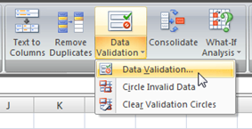Data Validation allows excel sheet users to specify what type of content a cell can hold or if it can hold something at all or not. With data validation in effect, the user can control generate an error message if the user try to enter something invalid or try to put something in cell that is not allowed for editing.

There are options available to allow entry of any value, whole numbers or floats, date and time, list, text length or a custom formula. The most useful option out of this is the list that allows user to select from a set of options. The next most useful option could be the one for entering integer numbers only. The custom formula allows you to set conditions using Excel’s build in formulas.

Understanding What If Analysis Tools

What if analysis Tools are a bunch of tools that are used to analyses scenario and what-if cases. There are three options available under it:

Scenario Manager, Goal Seek and the Data Tables. The scenario manager creates scenarios by asking user for the variables to be changed and naming them as different scenarios. The user keep naming the scenario and referring to the cells whose value will be changed resulting in a list of scenarios to be used.
The Goal seek option works by iterating through values until certain requirement is meet – for example if you set up a sheet with a formula where you wanted variable X to be 200 for some value of variable Y, the goal seek will keep iterating until it reaches corresponding value of Y.
The Data Table is good when you want to have more then one scenario to be displayed at once. Infect you can have a single scenario like displayed by scenario manager.
Repeating Last Action Quickly:

The easiest way to repeat the last action is to press F4. If you have formatted a cell with yellow fill and you want another cell to be formatted the same way, just press F4. If you have copied something and wanted to paste on multiple cells, select them and press F4.

Selecting Certain Type of Cells Only:

A Spreadsheet contains formulas, numbers, text and blank or non blank cells. We may want select only cells that belong to certain type for example only cells with formulas or only blank cells. In such situation the option of “Go To” is really handy.

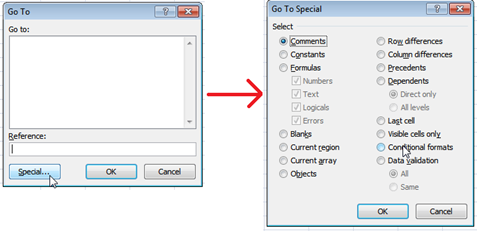The option can be found by pressing F5 that will ask you what to select. You can select more than one choices at a time as well. For example you want to select all the blank cell and put text “absent” on each of them. You will press F5, select blank that will select all the blank cells, write “absent” and will press ctrl+enter to have it in all selected cells.

Printing Sheet With Grid Lines and Headers:

When you are tired to starring at PC’s screen and want to have break, it is good idea to print you sheet focus on paper version of your sheet. But simply printing a sheet will not be of much help as there will be no header row and column to understand the formulas.

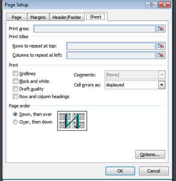It is possible to print a sheet with header row and column and grid lines with following options from print preview > page layout menu: